How To Do Vlookup In Excel With Two Spreadsheets

Vlookup between two workbooks / Vlookup between multiple worksheets

Below is an example of a vlookup between two unlike workbooks, which a lot of yous take been asking virtually.

To make information technology equally piece of cake as possible for you to sympathize the steps, we've included the two files we use for this free excel vlookup tutorial hither: Workbook without prices and Workbook with prices.

You lot can't learn how to drive a auto by merely reading a book, and for that reason, we've given you admission to the files that nosotros employ – after all, the all-time style to learn is by doing! Other sites practice non offer you the files, simply we practice. Nosotros recommend that you have both files open earlier you begin the tutorial.

The workbooks contain a list of products which the majority of people would purchase in a supermarket – Milk, Staff of life, Jam, etc.

We take intentionally kept the files uncomplicated. Nosotros're going to utilise the vlookup function to get the prices of the food data from the "workbook with prices" into the "workbook without prices".

Stride one

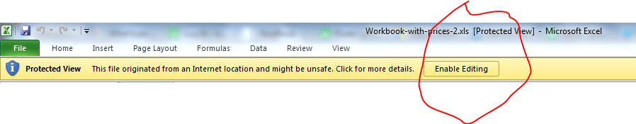
Earlier you start, open both workbooks from this site AND brand sure you've clicked the "Enable editing" push in BOTH workbooks and so save them to your Desktop, otherwise whatsoever changes you make won't piece of work!

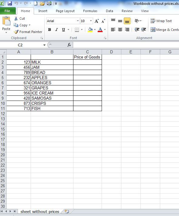
When yous open the "workbook without prices" file you volition meet the screen beneath. Cavalcade C in this workbook is where nosotros will pull in the "Cost of the Goods" from the other workbook. Cell C2 in the "workbook without prices" will already be selected – if it isn't, click in cell C2, as that'south where we want the kickoff result to appear.

An image showing a list of foods in column B with unique IDs in column A, but not cost information in col. C

Step 2

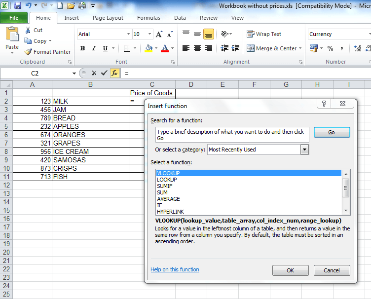
Click on the "fx" button which is just above cavalcade B (see screenshot below). The 'Insert Function' window will then bear witness up (also shown in the screenshot below). If the "vlookup function" is already selected, like in the screenshot below, click "ok".

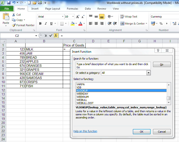
An image showing the Most Recently Used functions, with the vlookup at the top.

If the "vlookup office isn't already selected, so in the "or select a category" field shown in the screenshot above, change the option in the drop-down from "about recently used" to "All" then whorl down until you get to the vlookup function, as shown in the screenshot beneath.

An image showing All functions in the

One time you've selected the "vlookup office" from the drop downward carte and clicked ok, the "Part Arguments" window will announced.

Step 3

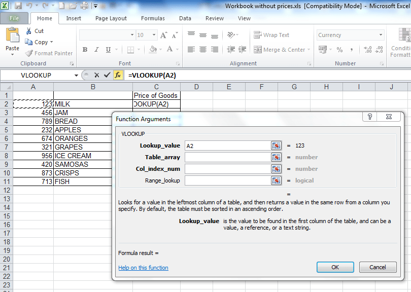
The "Function Arguments" window will bear witness 4 dissimilar fields which need to be populated for the vlookup to piece of work. For the first field, the "Lookup_value", click on cell A2, as illustrated in the image beneath.

The

Step 4

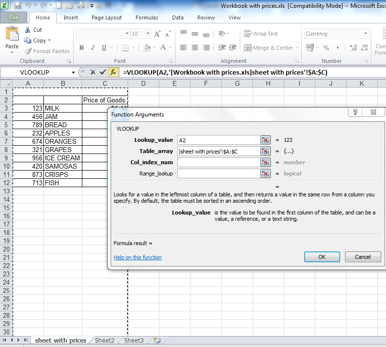
At present click into the "Table_array" field (a "table array" is a fancy phrase for describing two or more than columns of information).

Step 5

This part is where the other workbook comes in! After you lot've clicked in the "Table_array" field, click into the other workbook (it'southward called "workbook with prices") and highlight columns A – C in that workbook. Nosotros highlight columns A – C in this workbook because cavalcade A has the "Lookup_value" that is in the "workbook without prices" and column C has the "Cost of Goods" information that we want to extract from this workbook. When you highlighted columns A – C, you lot may take noticed that the characters "3C" appeared at the top of cavalcade D – this is a quick way of Excel telling you how many columns in that location are in the data you've highlighted – it saves you having to count the columns manually, which a lot of people in offices do! If y'all didn't detect that, clear the data in the "table assortment" field and highlight columns A – C again in the "workbook with prices" – ensure you concur the mouse fundamental as equally shortly as you let become, the "3C" volition disappear. Many office workers don't know this play a trick on and waste material a lot of time manually counting the columns! But nosotros're here to save you time!

NB – an alternative, but IMPORTANT way to populate the "Table_array" field is to highlight the range of data y'all're looking upwards, starting with your start unique value – in this case cell A3. And so you'd highlight cells A3 to C12, because C12 is the last cell in the range. You lot'd and then demand to Ready this table assortment by putting dollar signs in before the H, before the two, before the J and earlier the 11, and so your formula at the end looks like this: =VLOOKUP(B2,$A$iii:$C$12,3,Imitation). If you're in the table array field and you press F4, then Excel volition exercise this automatically for you lot.This is useful to know if a spreadsheet at work doesn't allow y'all to highlight columns A to C because some cells are merged or you lot're getting an invalid mistake. Only for now, just leave it, ensure, you're fields look the aforementioned as those in the screenshot beneath and so proceed to Step 6, the 2nd terminal stride.

The

Step 6

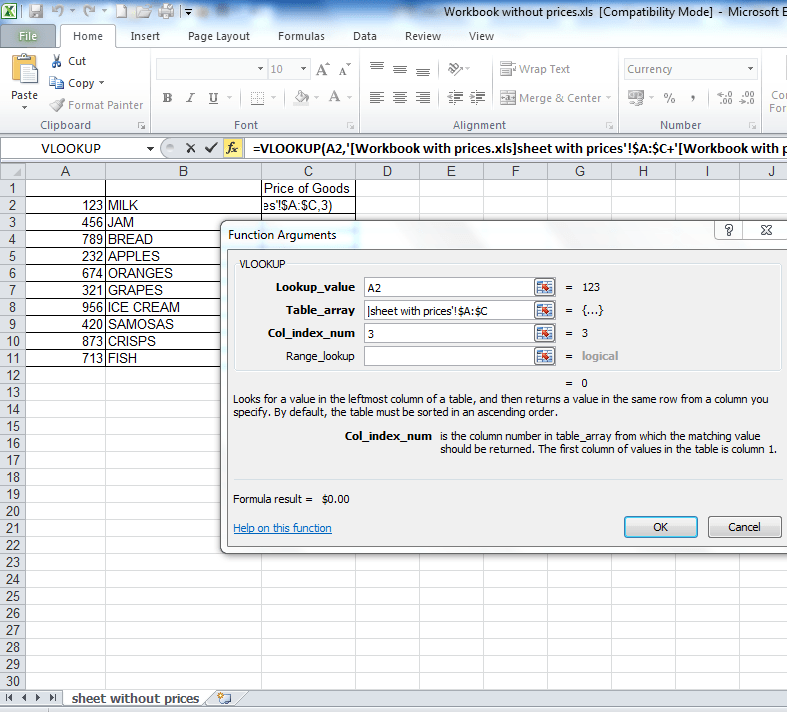
Click into the "Col_index_num" field – you will find that your screen returns back to the beginning file, the "workbook without prices" – don't panic! All you have to do here is put in the number 3. We put in the number 3 hither because column C in the "workbook with prices" has the prices of the appurtenances that we want and it is three columns abroad from column A, which has the unique lookup values that we are using. Or if yous noticed the "3C", information technology ways "three columns" so you know you have to insert the number iii in the "Col_index_num" field. A screenshot of how everything should expect so far is beneath.

The

Step vii

The final step! Click into the 'range lookup field' and type the discussion 'False'. Click 'OK' and, like magic, the formula will render the offset result that we're looking up. Afterwards that, just drag down the formula in cell C2 in the "workbook without prices" and the "prices" of all the other goods in this file will machine-populate. Piece of cake, right!? Typing the word 'FALSE' here volition ensure that the vlookup just returns an Exact match. If it doesn't find an verbal match for the 'lookup value' nosotros're using, then information technology will render an N/A – more virtually this in the "ten common problems" page above.

Your formula in the end should expect similar this (in jail cell C2 in the workbook without prices): =VLOOKUP(A2,'[Workbook-with-prices.xls]Sheet1′!$A:$C,3,FALSE)

If your formula does not look like this, then you lot need to check that yous've followed the steps above correctly.

iii people said they couldn't get to the 2nd workbook in step 5. This is because they hadn't clicked on the 'enable editing' push shown in the screenshots at the beginning of this tutorial in BOTH workbooks! Please brand sure you lot exercise this if this trouble applied to you, before posting a comment. In fact, you should ALWAYS click 'enable editing' if you're using formulas in Excel. Information technology's practiced exercise and will help you lot.

If you desire to learn about Pin Tables, you can practise so via this website we created following user demand: http://pivottablesinexcel.com/

If you lot accept issues with your vlookup click here – 13 common bug:

Nosotros ask that you lot accept a moment to read our Terms and Conditions and Privacy Policies.